Some Processes Do Not Follow One Straight Path
A simple sequence always moves to the next action.
Real programs often need to choose among possible paths.
Consider a soccer process:
The next action depends on a true/false condition.
If the player is available, the system may add the player to the available list.
If the player is not available, the system may leave the player off that list.
The process now contains a decision.
A Decision Node Represents a Choice in the Flow
In a UML activity diagram, a decision node represents a point where one incoming flow can continue along different outgoing paths.
Conceptually:
![Activity diagram showing ┌ [available] Add player to available list, then Read status ◇, then [not available] Continue without adding player.](Diagrams/0.3.ActivitiyDiagramDecisionBlocks.Activity.NodeRepresentsChoiceFlow.light.svg) AvailableAddPlayerToAvailableList.
AvailableAddPlayerToAvailableList.
The diamond represents the decision point.
The outgoing paths represent possible results.
Only the path whose condition is satisfied should be followed.
The Conditions on Paths Explain the Choice
The labels on the outgoing paths are often called guards.
They tell the reader when each path applies.
For the soccer example:
- [available]
- [not available]
A reader should be able to understand why one path is followed instead of the other.
Without path conditions, a decision diamond with two arrows would leave the choice unexplained.
Connect Decisions to Boolean Thinking
A decision often depends on a condition that can be understood as true or false.
Suppose the model tracks:
isAvailable
The process asks:
If the condition is true, follow the available path.
If it is false, follow the other path.
This is the same Boolean reasoning from the previous activity, now represented visually.
Paths Should Lead to Meaningful Actions
Consider:
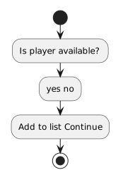 IsPlayerAvailable.
The diagram should make the consequence of the decision visible.
A decision whose two paths immediately do exactly the same thing may not be useful.
The point of branching is that the condition affects what happens next.
A Path Can Rejoin Later
Two paths do not have to remain separate forever.
For example:
![Activity diagram showing ┌ [available] Add to available list ┐, then Read availability ◇ Display roster, then [not available] ┘.](Diagrams/0.3.ActivitiyDiagramDecisionBlocks.Activity.PathCanRejoinLater.light.svg) AvailableAddToAvailableList.
AvailableAddToAvailableList.
Both paths eventually continue to Display roster.
The difference is that only the available path performs the extra action first.
This helps you see the difference between:
- a decision that changes part of the process;
- and the common work that happens afterward.
Keep the Decision Focused
A beginner diagram becomes difficult to read when one decision tries to answer several unrelated questions at once.
Instead of:
begin with the specific condition the current process actually needs.
For example:
Additional decisions can be modeled separately when the requirements call for them.
The Diagram Should Tell a Complete Story
A useful decision flow includes enough context to understand:
- what happened before the decision;
- what question controls the choice;
- what each path means;
- what happens on each path;
- and where the process goes afterward.
For example:
![Activity diagram showing Start, then Read player availability, then Decision: available?, then [yes] Add player to available list, then [no] Skip addition, then Display roster.](Diagrams/0.3.ActivitiyDiagramDecisionBlocks.Activity.ShouldTellCompleteStory.light.svg) Start.
Start.
The exact UML rendering may use standardized shapes rather than this text layout, but the meaning should remain the same.
Do Not Confuse the Decision With the Action
The decision asks a question.
The path condition identifies which result applies.
The next action performs work.
For example:
Decision: Is the player available?
Path: [yes]
Action: Add player to available list.
Keeping those roles separate makes both UML and later C# conditional logic easier to understand.
Follow One Path at a Time
When reading a decision diagram, choose a specific state.
Suppose:
isAvailable = true
Begin at the start node and trace only the path that applies to that state.
Then imagine:
isAvailable = false
Trace the other path.
This lets you treat the activity diagram as a description of possible execution paths rather than as a picture where everything happens at once.
From Diagram Decisions to Program Decisions
An activity diagram gives you a visual model of a choice.
C# later expresses the same kind of choice with conditional statements.
The syntax will look different, but the reasoning remains:
Evaluate a condition → select the matching path → continue execution
For now, focus on reading and creating that logic visually.