An Extensive Examination of Data Structures Using C# 2.0
Scott Mitchell 4GuysFromRolla.com
Update January 2005
Summary: This article, the third in a six-part series on data structures in the .NET Framework, looks at a common data structure that is not included in the .NET Framework Base Class Library—binary trees. Whereas arrays arrange data linearly, binary trees can be envisioned as storing data in two dimensions. A special kind of binary tree, called a binary search tree, or BST, allows for a much more optimized search time than with unsorted arrays. (30 printed pages)
Contents
Introduction Arranging Data in a Tree Understanding Binary Trees Improving the Search Time with Binary Search Trees (BSTs) Binary Search Trees in the Real-World
Introduction
In Part 1, we looked at what data structures are, how their performance can be evaluated, and how these performance considerations play into choosing which data structure to utilize for a particular algorithm. In addition to reviewing the basics of data structures and their analysis, we also looked at the most commonly used data structure, the array, and its relative, the List. In Part 2 we looked at the cousins of the List, the Stack and the Queue, which store their data like a List, but limit the means by which their contained data can be accessed. In Part 2 we also looked at the Hashtable and Dictionary classes, which are essentially arrays that are indexed by some arbitrary object as opposed to by an ordinal value.
The List, Stack, Queue, Hashtable, and Dictionary all use an underlying array as the means by which their data is stored. This means that, under the covers, these data structures are bound by the limitations imposed by an array. Recall from Part 1 that an array is stored linearly in memory, requires explicit resizing when the array's capacity is reached, and suffers from linear searching time.
In this third installment of the article series, we will examine a new data structure, the binary tree. As we'll see, binary trees store data in a non-linear fashion. After discussing the properties of binary trees, we'll look at a more specific type of binary tree—the binary search tree, or BST. A BST imposes certain rules on how the items of the tree are arranged. These rules provide BSTs with a sub-linear search time.
Arranging Data in a Tree
If you've ever looked at a genealogy table, or at the chain of command in a corporation, you've seen data arranged in a tree. A tree is composed of a collection of nodes, where each node has some associated data and a set of children. A node's children are those nodes that appear immediately beneath the node itself. A node's parent is the node immediately above it. A tree's root is the single node that contains no parent.
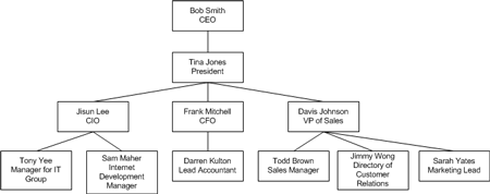
Figure 1 shows an example of the chain of command in a fictional company.
Figure 1. Tree view of a chain of command in a fictitious company
In this example, the tree's root is Bob Smith, CEO. This node is the root because it has no parent. The Bob Smith node has one child, Tina Jones, President, whose parent is Bob Smith. The Tina Jones node has three children—Jisun Lee, CIO; Frank Mitchell, CFO; and Davis Johnson, VP of Sales. Each of these nodes' parent is the Tina Jones node. The Jisun Lee node has two children—Tony Yee and Sam Maher; the Frank Mitchell node has one child—Darren Kulton; and the Davis Johnson node has three children—Todd Brown, Jimmy Wong, and Sarah Yates.
All trees exhibit the following properties:
There is precisely one root.
All nodes except the root have precisely one parent.
There are no cycles. That is, starting at any given node, there is not some path that can take you back to the starting node. The first two properties—that there exists one root and that all nodes save the root have one parent—guarantee that no cycles exist.
Trees are useful for arranging data in a hierarchy. As we will discuss later in this article, the time to search for an item can be drastically reduced by intelligently arranging the hierarchy. Before we can arrive at that topic, though, we need to first discuss a special kind of tree, the binary tree.
Understanding Binary Trees
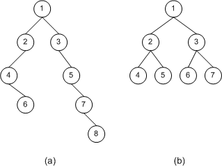
A binary tree is a special kind of tree, one in which all nodes have at most two children. For a given node in a binary tree, the first child is referred to as the left child, while the second child is referred to as the right child. Figure 2 depicts two binary trees.
Figure 2. Illustration of two binary trees
Binary tree (a) has 8 nodes, with node 1 as its root. Node 1's left child is node 2; node 1's right child is node 3. Notice that a node doesn't need to have both a left child and right child. In binary tree (a), node 4, for example, has only a right child. Furthermore, a node can have no children. In binary tree (b), nodes 4, 5, 6, and 7 all have no children.
Nodes that have no children are referred to as leaf nodes. Nodes that have one or two children are referred to as internal nodes. Using these new definitions, the leaf nodes in binary tree (a) are nodes 6 and 8; the internal nodes are nodes 1, 2, 3, 4, 5, and 7.
Unfortunately, the .NET Framework does not contain a binary tree class, so in order to better understand binary trees, let's take a moment to create our own binary tree class.
The First Step: Creating a Base Node Class
The first step in designing our binary tree class is to create a class that represents the nodes of the binary tree. Rather than create a class specific to nodes in a binary tree, let's create a base `Node` class that can be extended to meet the needs of a binary tree node through inheritance. The base `Node` class represents a node in a general tree, one whose nodes can have an arbitrary number of children. To model this, we'll create not just a `Node` class, but a `NodeList` class as well. The Node class contains some data and a NodeList instance, which represents the node's children. The `Node` class affords a perfect time to utilize the power of Generics, which will allow us to let the developer using the class decide at develop-time what type of data to store in the node.
Note that the `Node` class has two private member variables:
`data`, of type `T`. This member variable contains the data stored in the node of the type specified by the developer using this class.
`neighbors`, of type `NodeList<T>`. This member variable represents the node's children.
The remainder of the class contains the constructors and the public properties, which provide access to the two member variables.
The `NodeList` class contains a strongly-typed collection of `Node<T>` instances. As the following code shows, the `NodeList` class is derived from the `Collection<T>` class in the `System.Collections.Generics` namespace. The `Collection<T>` class provides the base functionality for a strong-typed collection, with methods like `Add(T)`, `Remove(T)`, and `Clear()`, and properties like `Count` and a default indexer. In addition to the methods and properties inherited from `Collection<T>`, `NodeList` provides a constructor that creates a specified number of nodes in the collection, and a method that searches the collection for an element of a particular value.
publicclassNodeList<T> : Collection<Node<T>>
{
publicNodeList() : base() { }
publicNodeList(int initialSize)
{
// Add the specified number of itemsfor (int i = 0; i < initialSize; i++)
base.Items.Add(default(Node<T>));
}
publicNode<T> FindByValue(T value)
{
// search the list for the valueforeach (Node<T> node in Items)
if (node.Value.Equals(value))
return node;
// if we reached here, we didn't find a matching nodereturnnull;
}
}
Extending the Base Node Class
While the `Node` class is adequate for any generic tree, a binary tree has tighter restrictions. As discussed earlier, a binary tree's nodes have at most two children, commonly referred to as left and right. To provide a binary tree-specific node class, we can extend the base Node class by creating a BinaryTreeNode class that exposes two properties—`Left` and `Right`—that operate on the base class's `Neighbors` property.
publicclassBinaryTreeNode<T> : Node<T>
{
publicBinaryTreeNode() : base() {}
publicBinaryTreeNode(T data) : base(data, null) {}
publicBinaryTreeNode(T data, BinaryTreeNode<T> left, BinaryTreeNode<T> right)
{
base.Value = data;
NodeList<T> children = newNodeList<T>(2);
children[0] = left;
children[1] = right;
base.Neighbors = children;
}
publicBinaryTreeNode<T> Left
{
get
{
if (base.Neighbors == null)
returnnull;
elsereturn (BinaryTreeNode<T>) base.Neighbors[0];
}
set
{
if (base.Neighbors == null)
base.Neighbors = newNodeList<T>(2);
base.Neighbors[0] = value;
}
}
publicBinaryTreeNode<T> Right
{
get
{
if (base.Neighbors == null)
returnnull;
elsereturn (BinaryTreeNode<T>) base.Neighbors[1];
}
set
{
if (base.Neighbors == null)
base.Neighbors = newNodeList<T>(2);
base.Neighbors[1] = value;
}
}
}
The lion's share of the work of this extended class is in the `Right` and `Left` properties. In these properties we need to ensure that the base class's `Neighbors` `NodeList` has been created. If it hasn't, then in the get accessor we return `null`; in the set accessor we need to create a new `NodeList` with precisely two elements. As you can see in the code, the `Left` property refers to the first element in the `Neighbors` collection (`Neighbors[0]`), while `Right` refers to the second (`Neighbors[1]`).
Creating the BinaryTree Class
With the `BinaryTreeNode` class complete, the `BinaryTree` class is a cinch to develop. The `BinaryTree` class contains a single private member variable—`root`. `root` is of type `BinaryTreeNode` and represents the root of the binary tree. This private member variable is exposed as a public property. (The `BinaryTree` class uses Generics as well; the type specified for the `BinaryTree` class is the type used for the `BinaryTreeNode` root.)
The `BinaryTree` class has a single public method, `Clear()`, which clears out the contents of the tree. `Clear()` works by simply setting the `root` to `null`. Other than the root and a `Clear()` method, the BinaryTree class contains no other properties or methods. Crafting the contents of the binary tree is the responsibility of the developer using this data structure.
The following code illustrates how to use the `BinaryTree` class to generate a binary tree with the same data and structure as binary tree (a) shown in Figure 2.
Note that we start by creating a `BinaryTree` class instance, and then create its root. We then must manually add new `BinaryTreeNode` class instances to the appropriate left and right children. For example, to add node 4, which is the left child of the left child of the root, we use: `btree.Root.Left.Left = new BinaryTreeNode<int>(4);`
Recall from Part 1 of this article series that an array's elements are stored in a contiguous block of memory. By doing so, arrays exhibit constant-time lookups. That is, the time it takes to access a particular element of an array does not change as the number of elements in the array increases.
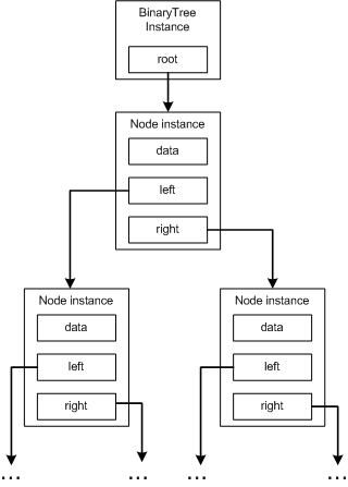
Binary trees, however, are not stored contiguously in memory, as Figure 3 illustrates. Rather, the `BinaryTree` class instance has a reference to the root `BinaryTreeNode` class instance. The root `BinaryTreeNode` class instance has references to its left and right child `BinaryTreeNode` instances; these child instances have references to their child instances, and so on. The point is, the various `BinaryTreeNode` instances that makeup a binary tree can be scattered throughout the CLR managed heap. They are not necessarily contiguous, as are the elements of an array.
Figure 3. Binary trees stored in memory
Imagine that we wanted to access a particular node in a binary tree. To accomplish this we need to search the binary tree's set of nodes, looking for the particular node. There's no direct access to a given node as with an array. Searching a binary tree can take linear time, as potentially all nodes will need to be examined. That is, as the number of nodes in the binary tree increases, the number of steps to find an arbitrary node will increase as well.
So, if a binary tree's lookup time is linear, and its search time is linear, how is the binary tree any better than an array, whose search time is linear, but whose lookup time is constant? Well, a generic binary tree doesn't offer us any benefit over an array. However, by intelligently organizing the items in a binary tree, we can greatly improve the search time (and therefore the lookup time as well).
Improving the Search Time with Binary Search Trees (BSTs)
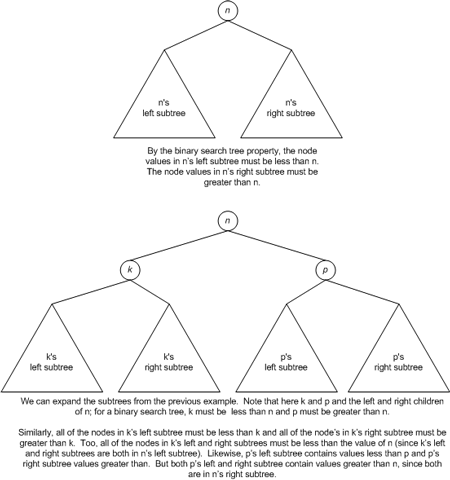
A binary search tree is a special kind of binary tree designed to improve the efficiency of searching through the contents of a binary tree. Binary search trees exhibit the following property: for any node n, every descendant node's value in the left subtree of n is less than the value of n, and every descendant node's value in the right subtree is greater than the value of n.
A subtree rooted at node n is the tree formed by imaging node n was a root. That is, the subtree's nodes are the descendants of n and the subtree's root is n itself. Figure 4 illustrates the concept of subtrees and the binary search tree property.
Figure 4. Subtrees and the binary search tree property
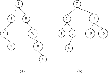
Figure 5 shows two examples of binary trees. The one on the right, binary tree (b), is a BST because it exhibits the binary search tree property. Binary tree (a), however, is not a BST because not all nodes of the tree exhibit the binary search tree property. Namely, node 10's right child, 8, is less than 10 but it appears in node 10's right subtree. Similarly, node 8's right child, node 4, is less than 8 but appears on node 8's right subtree. This property is violated in other locations, too. For example, node 9's right subtree contains values less than 9, namely 8 and 4.
Figure 5. Comparison of non-BST binary tree (a) and a BST binary tree (b)
Note that for the binary search tree property to be upheld, the data stored in the nodes of a BST must be able to be compared to one another. Specifically, given two nodes, a BST must be able to determine if one is less than, greater than, or equal to the other.
Now, imagine that you want to search a BST for a particular node. For example, for the BST in Figure 5 (the binary tree (b)), imagine that we wanted to search for the node 10. A BST, like a regular binary tree, only has a direct reference to one node, its root. Can you think of an optimal way to search the tree to see if node 10 exists? There's a better way than searching through each node in the tree.
To see if 10 exists in the tree we can start with the root. We see that the root's value (7) is less than the value of the node we are looking for. Therefore, if 10 does exist in the BST, it must be in the root's right subtree. Therefore, we continue our search at node 11. Here we notice that 10 is less than 11, so if 10 exists in the BST it must exist in the left subtree of 11. Moving onto the left child of 11, we find node 10, and have located the node we are looking for.
What happens if we search for a node that does not exist in the tree? Imagine that we wanted to find node 9. We'd start by repeating the same steps above. Upon reaching node 10, we'd see that node 10 was greater than 9, so 9, if it exists, must be in 10's left subtree. However, we'd notice that 10 has no left child, therefore 9 must not exist in the tree.
More formally, our searching algorithm goes as follows. We have a node n we wish to find (or determine if it exists), and we have a reference to the BST's root. This algorithm performs a number of comparisons until a null reference is hit or until the node we are searching for is found. At each step we are dealing with two nodes: a node in the tree, call it c, that we are currently comparing with n, the node we are looking for. Initially, c is the root of the BST. We apply the following steps:
If c is a null reference, then exit the algorithm. n is not in the BST.
Compare c's value and n's value.
If the values are equal, then we found n.
If n's value is less than c's then n, if it exists, must be in the c's left subtree. Therefore, return to step 1, letting c be c's left child.
If n's value is greater than c's then n, if it exists, must be in the c's right subtree. Therefore, return to step 1, letting c be c's right child.
We applied these steps earlier when searching for node 10. We started with the root node and noted that 10 was greater than 7, so we repeated our comparison with the root's right child, 11. Here, we noted 10 was less than 11, so we repeated our comparison with 11's left child. At this point we had found node 10. When searching for node 9, which did not exist, we wound up performing our comparison with 10's left child, which was a null reference. Hence we deduced that 9 did not exist in the BST.
Analyzing the BST Search Algorithm
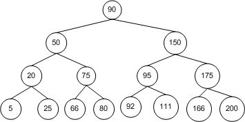
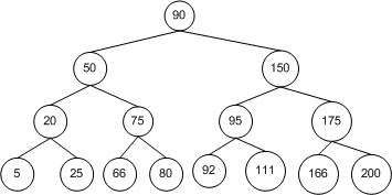
For finding a node in a BST, at each stage we ideally reduce the number of nodes we have to check by half. For example, consider the BST in Figure 6, which contains 15 nodes. When starting our search algorithm at the root, our first comparison will take us to either the root's left or right child. In either case, once this step is made the number of nodes that need to be considered has just halved, from 15 down to 7. Similarly, at the next step the number is halved again, from 7 down to 3, and so on.
Figure 6. BST with 15 nodes
The important concept to understand here is that ideally at each step in the algorithm the number of nodes that have to be considered has been cut in half. Compare this to searching an array. When searching an array we have to search all elements, one element at a time. That is, when searching an array with n elements, after we check the first element, we still have n – 1 elements to check. With a BST of n nodes, however, after checking the root we have whittled the problem down to searching a BST with n/2 nodes.
Searching a binary tree is similar in analysis to searching a sorted array. For example, imagine you wanted to find if there is a John King in the phonebook. You could start by flipping to the middle of the phone book. Here, you'd likely find people with last names starting with the letter M. Because K comes before M alphabetically, you would then flip halfway between the start of the phonebook and the page you had reached in the Ms. Here, you might end up in the Hs. Since K comes after H, you'd flip half way between the Hs and the Ms. This time you might hit the Ks, where you could quickly see if James King was listed.
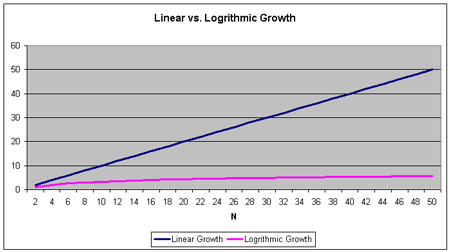
This is similar to searching a BST. With an ideally arranged BST the midpoint is the root. We then traverse down the tree, navigating to the left and right children as needed. These approaches cut the search space in half at each step. Such algorithms that exhibit this property have an asymptotic running time of log2 n, commonly abbreviated lg n. Recall from our mathematical discussions in Part 1 of this article series that log2 n = y means that 2y = n. That is, as n grows, log2 n grows very slowly. The growth rate of log2 n compared to linear grown is shown in the graph in Figure 7. Due to log2 n's slower growth than linear time, algorithms that run in asymptotic time log2 n are said to be sublinear.
Figure 7. Comparison of linear growth rate vs. log 2 n
While it may appear that the logarithmic curve is flat, it is increasing, albeit rather slowly. To appreciate the difference between linear and sublinear growth, consider searching an array with 1,000 elements versus searching a BST with 1,000 elements. For the array, we'll have to search up to 1,000 elements. For the BST, we'd ideally have to search no more than ten nodes! (Note that log10 1024 equals 10.)
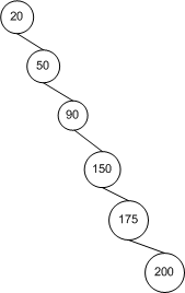
Throughout our analysis of the BST search algorithm, I've repeatedly used the word "ideally." This is because the search time for a BST depends upon its topology, or how the nodes are laid out with respect to one another. For a binary tree like the one in Figure 6, each comparison stage in the search algorithm trims the search space in half. However, consider the BST shown in Figure 8, whose topology is synonymous to how an array is arranged.
Figure 8. Example of BST that will be searched in linear time
Searching the BST in Figure 8 will take linear time because after each comparison the problem space is only reduced by 1 node, not by half of the current nodes, as with the BST in Figure 6.
Therefore, the time it takes to search a BST is dependent upon its topology. In the best case, the time is on the order of log2 n, but in the worst case it requires linear time. As we'll see in the next section, the topology of a BST is dependent upon the order with which the nodes are inserted. Therefore, the order with which the nodes are inserted affects the running time of the BST search algorithm.
Inserting Nodes into a BST
We've seen how to search a BST to determine if a particular node exists, but we've yet to look at how to add a new node. When adding a new node we can't arbitrarily add the new node; rather, we have to add the new node such that the binary search tree property is maintained.
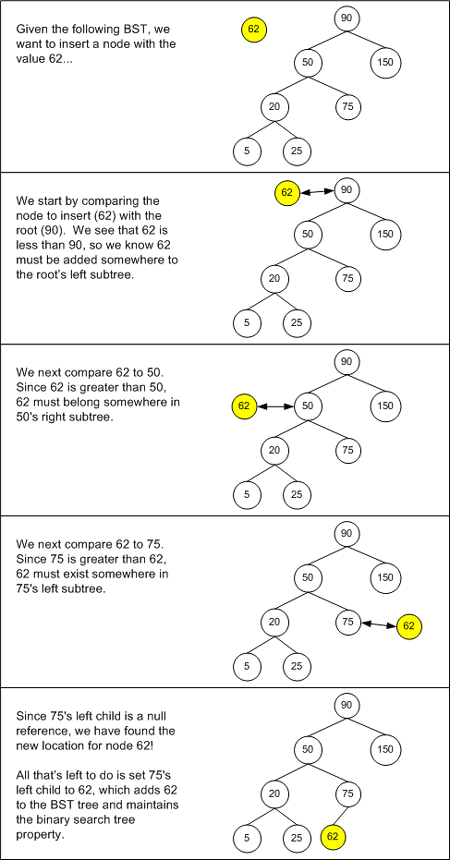
When inserting a new node we will always insert the new node as a leaf node. The only challenge, then, is finding the node in the BST which will become this new node's parent. Like with the searching algorithm, we'll be making comparisons between a node c and the node to be inserted, n. We'll also need to keep track of c's parent node. Initially, c is the BST root and parent is a null reference. Locating the new parent node is accomplished by using the following algorithm:
If c is a null reference, then parent will be the parent of n. If n's value is less than parent's value, then n will be parent's new left child; otherwise n will be parent's new right child.
Compare c and n's values.
If c's value equals n's value, then the user is attempting to insert a duplicate node. Either simply discard the new node, or raise an exception. (Note that the nodes' values in a BST must be unique.)
If n's value is less than c's value, then n must end up in c's left subtree. Let parent equal c and c equal c's left child, and return to step 1.
If n's value is greater than c's value, then n must end up in c's right subtree. Let parent equal c and c equal c's right child, and return to step 1.
This algorithm terminates when the appropriate leaf is found, which attaches the new node to the BST by making the new node an appropriate child of parent. There's one special case you have to worry about with the insert algorithm: if the BST does not contain a root, then there parent will be null, so the step of adding the new node as a child of parent is bypassed; furthermore, in this case the BST's root must be assigned to the new node.
Figure 9 depicts the BST insert graphically.
Figure 9. Insert into a BST
Both the BST search and insert algorithms share the same running time—log2 n in the best case, and linear in the worst case. The insert algorithm's running time mimics the search's because it, essentially, uses the same tactics used by the search algorithm to find the location for the newly inserted node.
The Order of Insertion Determines the BST's Topology
Since newly inserted nodes into a BST are inserted as leaves, the order of insertion directly affects the topology of the BST itself. For example, imagine we insert the following nodes into a BST: 1, 2, 3, 4, 5, and 6. When 1 is inserted, it is insert as the root. Next, 2 is inserted as 1's right child. 3 is inserted as 2's right child, 4 as 3's right child, and so on. The resulting BST is one whose structure is precisely that of the BST in Figure 8.
If the values 1, 2, 3, 4, 5, and 6 had been inserted in a more intelligent manner, the BST would have had more breadth, and would have looked more like the tree in Figure 6. The ideal insertion order would be: 4, 2, 5, 1, 3, 6. This would put 4 at the root, 2 as 4's left child, 5 as 4's right child, 1 and 3 as 2's left and right children, and 6 as 5's right child.
Because the topology of a BST can greatly affect the running time of search, insert, and (as we will see in the next section) delete, inserting data in ascending or descending order (or in near order) can have devastating results on the efficiency of the BST. We'll discuss this topic in more detail at the article's end, in the "Binary Search Trees in the Real-World" section.
Deleting Nodes from a BST
Deleting nodes from a BST is slightly more difficult than inserting a node because deleting a node that has children requires that some other node be chosen to replace the hole created by the deleted node. If the node to replace this hole is not chosen with care, the binary search tree property may be violated. For example, consider the BST in Figure 6. If the node 150 is deleted, some node must be moved to the hole created by node 150's deletion. If we arbitrarily choose to move, say node 92 there, the BST property is deleted since 92's new left subtree will have nodes 95 and 111, both of which are greater than 92 and thereby violating the binary search tree property.
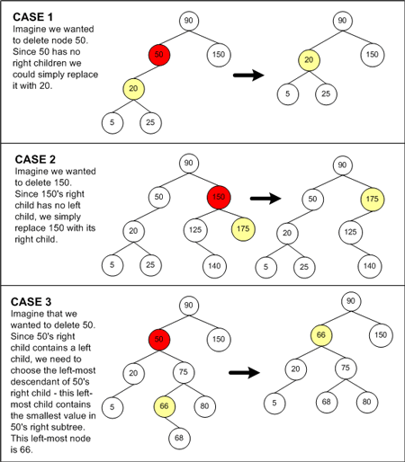
The first step in the algorithm to delete a node is to first locate the node to delete. This can be done using the searching algorithm discussed earlier, and therefore has a log2 n running time. Next, a node from the BST must be selected to take the deleted node's position. There are three cases to consider when choosing the replacement node, all of which are illustrated in Figure 10.
Case 1: If the node being deleted has no right child, then the node's left child can be used as the replacement. The binary search tree property is maintained because we know that the deleted node's left subtree itself maintains the binary search tree property, and that the values in the left subtree are all less than or all greater than the deleted node's parent, depending on whether the deleted node is a left or right child. Therefore, replacing the deleted node with its left subtree will maintain the binary search tree property.
Case 2: If the deleted node's right child has no left child, then the deleted node's right child can replace the deleted node. The binary search tree property is maintained because the deleted node's right child is greater than all nodes in the deleted node's left subtree and is either greater than or less than the deleted node's parent, depending on whether the deleted node was a right or left child. Therefore, replacing the deleted node with its right child will maintain the binary search tree property.
Case 3: Finally, if the deleted node's right child does have a left child, then the deleted node needs to be replaced by the deleted node's right child's left-most descendant. That is, we replace the deleted node with the deleted node's right subtree's smallest value. **Note **Realize that for any BST, the smallest value in the BST is the left-most node, while the largest value is the right-most node. This replacement choice maintains the binary search tree property because it chooses the smallest node from the deleted node's right subtree, which is guaranteed to be larger than all node's in the deleted node's left subtree. Too, since it's the smallest node from the deleted node's right subtree, by placing it at the deleted node's position, all of the nodes in its right subtree will be greater.
Figure 10 illustrates the node to choose for replacement for each of the three cases.
Figure 10. Cases to consider when deleting a node
As with the insert and searching algorithms, the asymptotic running time of delete is dependent upon the BST's topology. Ideally, the running time is on the order of log2 n. However, in the worst case, it takes linear time.
Traversing the Nodes of a BST
With the linear, contiguous ordering of an array's elements, iterating through an array is a straightforward manner: start at the first array element, and step through each element sequentially. For BSTs there are three different kinds of traversals that are commonly used:
Preorder traversal
Inorder traversal
Postorder traversal
Essentially, all three traversals work in roughly the same manner. They start at the root and visit that node and its children. The difference among these three traversal methods is the order with which they visit the node itself versus visiting its children. To help clarify this, consider the BST in Figure 11. (Note that the BST in Figure 11 is the same as the BST in Figure 6 and is repeated here for convenience.)
Figure 11. A sample Binary Search Tree
Preorder Traversal
Preorder traversal starts by visiting the current node—call it c—then its left child, and then its right child. Starting with the BST's root as c, this algorithm can be written out as:
Visit c. This might mean printing out the value of the node, adding the node to a List, or something else. It depends on what you want to accomplish by traversing the BST.
Repeat step 1 using c's left child.
Repeat step 1 using c's right child.
Imagine that in step 1 of the algorithm we were printing out the value of c. In this case, what would the output be for a preorder traversal of the BST in Figure 11? Well, starting with step 1 we would print the root's value. Step 2 would have us repeat step 1 with the root's left child, so we'd print 50. Step 2 would have us repeat step 1 with the root's left child's left child, so we'd print 20. This would repeat all the way down the left side of the tree. When 5 was reached, we'd first print out its value (step 1). Since there are no left or right children of 5, we'd return to node 20, and perform its step 3, which is repeating step 1 with 20's right child, or 25. Since 25 has no children, we'd return to 20, but we've done all three steps for 20, so we'd return to 50, and then take on step 3 for node 50, which is repeating step 1 for node 50's right child. This process would continue on until each node in the BST had been visited. The output for a preorder traversal of the BST in Figure 11 would be: 90, 50, 20, 5, 25, 75, 66, 80, 150, 95, 92, 111, 175, 166, 200.
Understandably, this may be a bit confusing. Perhaps looking at some code will help clarify things. The following code shows a method to iterate through the items of BST in a preorder traversal. Note that this method takes in a `BinaryTreeNode` class instance as one of its input parameters. This input node is the node c from the list of the algorithm's steps. Realize that a preorder traversal of the BST would begin by calling this method, passing in the BST's root.
void PreorderTraversal(Node current)
{
   if (current != null)
   {
            // Output the value of the current node
      Console.WriteLine(current.Value);

            // Recursively print the left and right children
      PreorderTraversal(current.Left);
      PreorderTraversal(current.Right);
   }
}
Inorder Traversal
Inorder traversal starts by visiting the current node's left child, then the current node, and then its right child. Starting with the BST's root as c, this algorithm can be written out as:
Repeat step 1 using c's left child.
Visit c. This might mean printing out the value of the node, adding the node to an ArrayList, or something else. It depends on what you want to accomplish by traversing the BST.
Repeat step 1 using c's right child.
The code for `InorderTraversal()` is just like `PreorderTraversal()` except that adding the `current` Node's data to the `StringBuilder` occurs after another call to `InorderTraversal()`, passing in `current`'s left child.
void InorderTraversal(Node current)
{
   if (current != null)
   {
            // Visit the left child...
      InorderTraversal(current.Left);

            // Output the value of the current node
      Console.WriteLine(current.Value);

            // Visit the right child...
      InorderTraversal(current.Right);
   }
}
Applying an inorder traversal to the BST in Figure 11, the output would be: 5, 20, 25, 50, 66, 75, 80, 90, 92, 95, 111, 150, 166, 175, 200. Note that the results returned are in ascending order.
Postorder Traversal
Finally, postorder traversal starts by visiting the current node's left child, then its right child, and finally the current node itself. Starting with the BST's root as c, this algorithm can be written out as:
Repeat step 1 using c's left child.
Repeat step 1 using c's right child.
Visit c. This might mean printing out the value of the node, adding the node to an ArrayList, or something else. It depends on what you want to accomplish by traversing the BST.
The output of a postorder traversal for the BST in Figure 11 would be: 5, 25, 20, 66, 80, 75, 50, 92, 111, 95, 166, 200, 175, 150, 90.
Realize that all three traversal times exhibit linear asymptotic running time. This is because each traversal option visits each and every node in the BST precisely once. So, if the number of nodes in the BST are doubled, the amount of work for a traversal doubles as well.
The Cost of Recursion
Recursive functions are often ideal for visualizing an algorithm, as they can often eloquently describe an algorithm in a few short lines of code. However, when iterating through a data structure's elements in practice, recursive functions are usually sub-optimal. Iterating through a data structure's elements involves stepping through the items and returning them to the developer utilizing the data structure, one at a time. Recursion is not suited to stopping abruptly at each step of the process. For this reason, the enumerator for the `BinarySearchTree` class uses a non-recursive solution to iterate through the elements.
Implementing a BST Class
The .NET Framework Base Class Library does not include a binary search tree class, so let's create one ourselves. The `BinarySearchTree` class can reuse the `BinaryTreeNode` class we examined earlier. Over the next few sections we'll look at each of the major methods of the class. For the class's full source code, be sure to download the source code that accompanies this article, which also includes a Windows Forms application for testing the BST class.
Searching for a Node
The reason BSTs are important to study is that they offer sublinear search times. Therefore, it only makes sense to first examine the BSTs `Contains()` method. The `Contains()` method accepts a single input parameter and returns a Boolean indicating if that value exists in the BST.
`Contains()` starts at the root and iteratively percolates down the tree until it either reaches a `null` reference, in which case `false` is returned, or until it finds the node being searched for, in which case `true` is returned. In the `while` loop, `Contains()` compares the `Value` of the current `BinaryTreeNode` instance against the data being searched for, and snakes its way down the right or left subtree accordingly. The comparison is performed by a private member variable, `comparer`, which is of type `IComparer<T>` (where `T` is the type defined via the Generics syntax for the BST). By default, `comparer` is assigned the default `Comparer` class for the type T, although the `BST` class's constructor has an overload to specify a custom `Comparer` class instance.
publicbool Contains(T data)
{
// search the tree for a node that contains dataBinaryTreeNode<T> current = root;
int result;
while (current != null)
{
result = comparer.Compare(current.Value, data);
if (result == 0)
// we found datareturntrue;
elseif (result > 0)
// current.Value > data, search current's left subtree
current = current.Left;
elseif (result < 0)
// current.Value < data, search current's right subtree
current = current.Right;
}
returnfalse; // didn't find data
}
Adding a Node to the BST
Unlike the `BinaryTree` class we created earlier, the `BinarySearchTree` class does not provide direct access to its root. Rather, nodes are added to the BST through the BST's `Add()` method. `Add()` takes as input the item to add to the BST, which is then percolated down the tree, looking for its new parent. (Recall that the any new nodes added to a BST will be added as leaf nodes.) Once the new node's parent is found, the node is made either the left or right child of the parent, depending on if its value is less than or greater than the parent's value.
publicvirtualvoidAdd(T data)
{
// create a new Node instanceBinaryTreeNode<T> n = newBinaryTreeNode<T>(data);
int result;
// now, insert n into the tree// trace down the tree until we hit a NULLBinaryTreeNode<T> current = root, parent = null;
while (current != null)
{
result = comparer.Compare(current.Value, data);
if (result == 0)
// they are equal - attempting to enter a duplicate - do nothingreturn;
elseif (result > 0)
{
// current.Value > data, must add n to current's left subtree
parent = current;
current = current.Left;
}
elseif (result < 0)
{
// current.Value < data, must add n to current's right subtree
parent = current;
current = current.Right;
}
}
// We're ready to add the node!
count++;
if (parent == null)
// the tree was empty, make n the root
root = n;
else
{
result = comparer.Compare(parent.Value, data);
if (result > 0)
// parent.Value > data, therefore n must be added to the left subtree
parent.Left = n;
else// parent.Value < data, therefore n must be added to the right subtree
parent.Right = n;
}
}
As you can see by examining the code, if the user attempts to add a duplicate the `Add()` method does nothing. That is, the BST cannot contain nodes with duplicate values. If you want, rather than simply returning, you could alter this code so inserting a duplicate raises an exception.
Deleting a Node from the BST
Recall that deleting a node from a BST is the trickiest of the BST operations. The trickiness is due to the fact that deleting a node from a BST necessitates that a replacement node be chosen to occupy the space once held by the deleted node. Care must be taken when selecting this replacement node so that the binary search tree property is maintained.
Earlier, in the "Deleting Nodes from a BST" section, we discussed how there were three different scenarios for deciding what node to choose to replace the deleted node. These cases were summarized in Figure 10. Below you can see how the cases are identified and handled in the `Remove()` method.
publicbool Remove(T data)
{
// first make sure there exist some items in this treeif (root == null)
returnfalse; // no items to remove// Now, try to find data in the treeBinaryTreeNode<T> current = root, parent = null;
int result = comparer.Compare(current.Value, data);
while (result != 0)
{
if (result > 0)
{
// current.Value > data, if data exists it's in the left subtree
parent = current;
current = current.Left;
}
elseif (result < 0)
{
// current.Value < data, if data exists it's in the right subtree
parent = current;
current = current.Right;
}
// If current == null, then we didn't find the item to removeif (current == null)
returnfalse;
else
result = comparer.Compare(current.Value, data);
}
// At this point, we've found the node to remove
count--;
// We now need to "rethread" the tree// CASE 1: If current has no right child, then current's left child becomes// the node pointed to by the parentif (current.Right == null)
{
if (parent == null)
root = current.Left;
else
{
result = comparer.Compare(parent.Value, current.Value);
if (result > 0)
// parent.Value > current.Value, so make current's left child a left child of parent
parent.Left = current.Left;
elseif (result < 0)
// parent.Value < current.Value, so make current's left child a right child of parent
parent.Right = current.Left;
}
}
// CASE 2: If current's right child has no left child, then current's right child// replaces current in the treeelseif (current.Right.Left == null)
{
current.Right.Left = current.Left;
if (parent == null)
root = current.Right;
else
{
result = comparer.Compare(parent.Value, current.Value);
if (result > 0)
// parent.Value > current.Value, so make current's right child a left child of parent
parent.Left = current.Right;
elseif (result < 0)
// parent.Value < current.Value, so make current's right child a right child of parent
parent.Right = current.Right;
}
}
// CASE 3: If current's right child has a left child, replace current with current's// right child's left-most descendentelse
{
// We first need to find the right node's left-most childBinaryTreeNode<T> leftmost = current.Right.Left, lmParent = current.Right;
while (leftmost.Left != null)
{
lmParent = leftmost;
leftmost = leftmost.Left;
}
// the parent's left subtree becomes the leftmost's right subtree
lmParent.Left = leftmost.Right;
// assign leftmost's left and right to current's left and right children
leftmost.Left = current.Left;
leftmost.Right = current.Right;
if (parent == null)
root = leftmost;
else
{
result = comparer.Compare(parent.Value, current.Value);
if (result > 0)
// parent.Value > current.Value, so make leftmost a left child of parent
parent.Left = leftmost;
elseif (result < 0)
// parent.Value < current.Value, so make leftmost a right child of parent
parent.Right = leftmost;
}
}
returntrue;
}
The `Remove()` method returns a Boolean to indicate whether or not the item was removed successfully from the binary search tree. False is returned in the case where the item to be removed was not found within the tree.
The Remaining BST Methods and Properties
There are a few other BST methods and properties not examined here in this article. Be sure to download this article's accompanying code for a complete look at the BST class. The remaining methods and properties are:
`Clear()`: removes all of the nodes from the BST.
`CopyTo(Array, index[, TraversalMethods]):`copies the contents of the BST to a passed-in array. By default, an inorder traversal is used, although a specific traversal method can be specified. The `TraversalMethods` enumeration options are `Preorder`, `Inorder`, and `Postorder`.
`GetEnumerator([TraversalMethods]):` provides iteration through the BST using inorder traversal, by default. Other traversal methods can be optionally specified.
`Count`: a public, read-only property that returns the number of nodes in the BST.
`Preorder`, `Inorder`, and `Postorder:` these three properties return `IEnumerable<T>` instances that can be used to enumerate the items in the BST in a specified traversal order.
The `BST` class implements the `ICollection`, `ICollection<T>`, `IEnumerable`, and `IEnumerable<T>` interfaces.
Binary Search Trees in the Real-World
While binary search trees ideally exhibit sublinear running times for insertion, searches, and deletes, the running time is dependent upon the BST's topology. The topology, as we discussed in the "Inserting Nodes into a BST" section, is dependent upon the order with which the data is added to the BST. Data being entered that is ordered or near-ordered will cause the BST's topology to resemble a long, skinny tree, rather than a short and fat one. In many real-world scenarios, data is naturally in an ordered or near-ordered state.
The problem with BSTs is that they can become easily unbalanced. A balaced binary tree is one that exhibits a good ratio of breadth to depth. As we will examine in the next part of this article series, there are a special class of BSTs that are self-balancing. That is, as new nodes are added or existing nodes are deleted, these BSTs automatically adjust their topology to maintain an optimal balance. With an ideal balance, the running time for inserts, searches, and deletes, even in the worst case, is log2 n.
In the next installment of this article series, we'll look at a couple self-balancing BST derivatives, including the red-black tree, and then focus on a data structure known as a SkipList, which exhibits the benefits of self-balancing binary trees, but without the need for restructuring the topology. Restructuring the topology, while efficient, requires a good deal of difficult code and is anything but readable.
Until then, happy programming!
Appendix A: Definitions
The following table is an alphabetized list of definitions for terms used throughout this article.
Binary tree: A tree where each node has at most two children.
Binary search tree: A binary tree that exhibits the following property: for any node n, every descendant node's value in the left subtree of n is less than the value of n, and every descendant node's value in the right subtree is greater than the value of n.
Cycle: A cycle exists if starting from some node n there exists a path that returns to n.
Internal node: A node that has one or more children.
Leaf node: A node that has no children.
Node: Nodes are the building blocks of trees. A node contains some piece of data, a parent, and a set of children. (Note: the root node does not contain a parent; leafnodes do not contain children.)
Root: The node that has no parent. All trees contain precisely one root.
Subtree: A subtree rooted at node n is the tree formed by imaging node n was a root. That is, the subtree's nodes are the descendants of n and the subtree's root is n itself.
Appendix B: Running Time Summaries
The following table lists the common operations that are performed on a BST and their associated running times.
Operation: Best Case Running Time
Search: log2n
Insert: log2n
Delete: log2n
Preorder Traversal:
Inorder Traversal:
Postorder Traversal:
References
Cormen, Thomas H., Charles E. Leiserson, and Ronald L. Rivest. "Introduction to Algorithms." MIT Press. 1990.
Scott Mitchell, author of six books and founder of 4GuysFromRolla.com, has been working with Microsoft Web technologies since January 1998. Scott works as an independent consultant, trainer, and writer, and holds a Masters degree in Computer Science from the University of California – San Diego. He can be reached at mitchell@4guysfromrolla.com, or via his blog at https://ScottOnWriting.NET
.